Real Simulation
1. Reach the job ordering page for your mesh
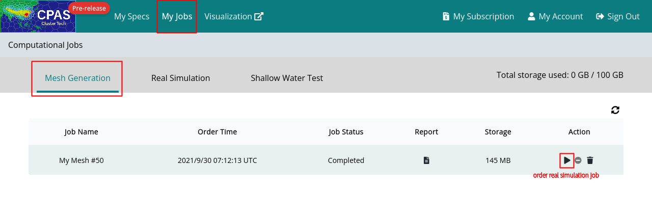
Click “My Jobs” at the navigation bar to display Computational Jobs, and select the “Mesh Generation” tab if it has not been selected, which lists all your mesh generation jobs and indicates their status. Once your desired mesh job is marked as “Completed”, you can click the play button ▶ at the right of the job item to order a real simulation for it.
2. Specify options for real simulation
The following sections are available for you to configure for your real simulation:
- Job particulars
- (Optional) Four-dimensional Data Assimilation (FDDA)
- (For limited-area mesh) Limited-area simulation
- CPAS model options
- Output files and variables to output
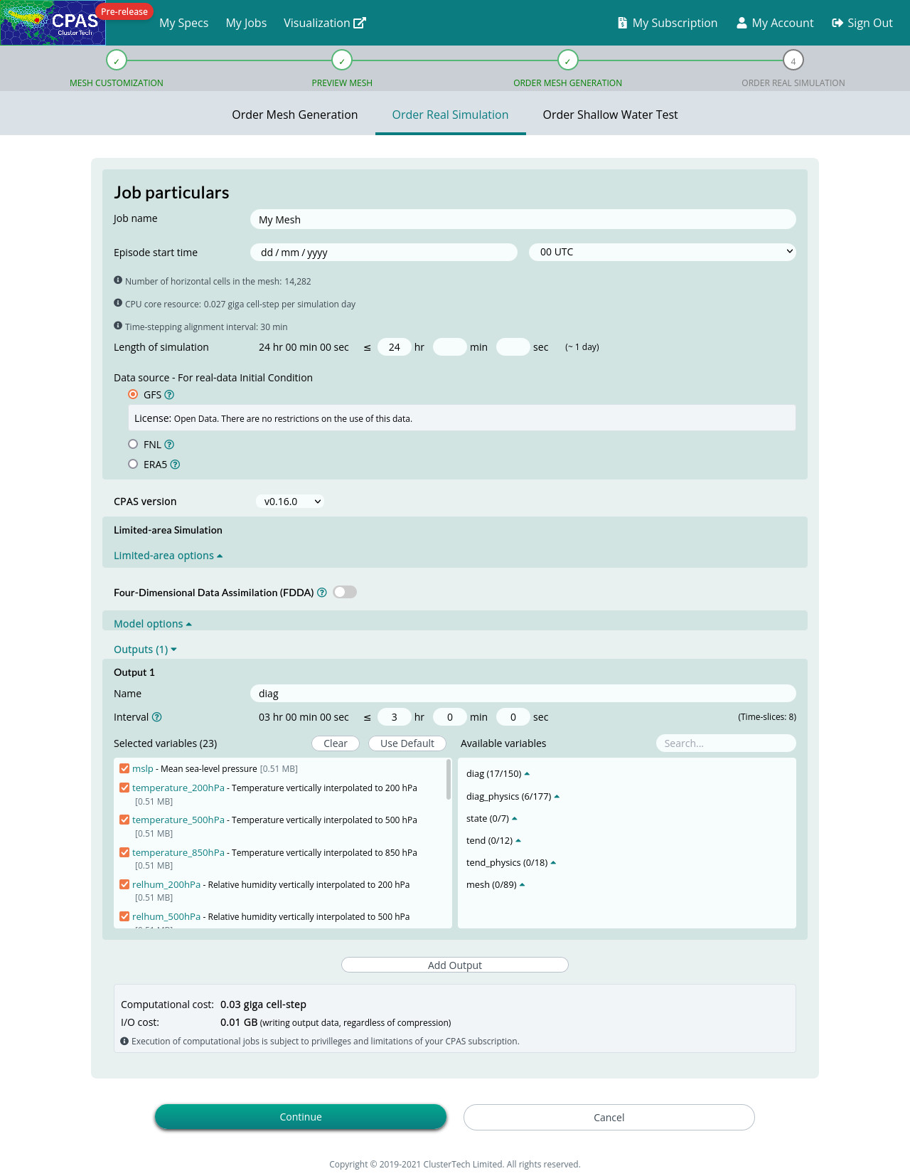
Job particulars
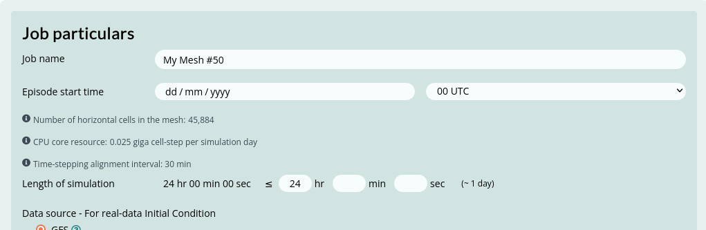
The Episode start time should be selected according to the availability of the data source. Four data updates are provided each day, namely at 00 UTC, 06 UTC, 12 UTC and 18 UTC (UTC means Coordinated Universal Time). Usually, there are more radiosonde ("weather balloon" sounding) observations in the 00 UTC and 12 UTC datasets and hence these two initial conditions are of higher quality.
|
Usual practice for running a meteorological model requires a spin-up time before simulation results can be regarded as valid. This is because of mismatches of grid and resolution between the initial condition and the running model, and the variables (especially those for classifying states of moisture) of the initial condition may not be fully compatible with the running model. In particular, for regions where the running model has finer resolution than the initial condition, a spin-up time is needed for the resolved terrain and land use data to take effect, and for micro-weather states to be generated. For a long spin-up time, observation data used for the initial condition is less informative, and a short spin-up time may introduce inaccuracies in the atmospheric state; from our experience, 12-18 hours is an appropriate choice for most practical uses. |
|
For example, if you would like to evaluate the model for a 5-day prediction, a 0.5 day spin-up is recommended, therefore setting Length of simulation (hours) to be 132 (=5.5*24). The computation cost needed is directly proportional to the length of simulation (for a fixed number of vertical layers, e.g. for a 0.39 giga cell-step per simulation day example, the computational cost for a 5.5-day simulation would be 0.39 * 5.5 = 2.145 giga cell-step.
|
Data source - For real-data Initial Condition
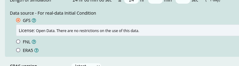
Three data sources are available. At present, all data are of 0.25 degree resolution.
| GFS | The US NCEP GFS forecast data product. The data is near real-time (several hours delay). GFS data since 2015-01-15 shall be available. |
| FNL | The US NCEP FNL (Final) Operational Global Analysis dataset. The data usually has one or two days of delay. FNL data since 2015-07-08 shall be available. |
| ERA5 | The ECMWF ERA5 reanalysis dataset. The data has a 5 days delay. ERA5 data since 1979 shall be available. |
For other initial conditions, it is not covered by the automated cloud-computing service. Please contact enquiry@cpas.earth.
CPAS model version
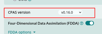
We have pre-selected the latest version for you, but you can select another particular version you want. Different versions may have different arrangements of options.
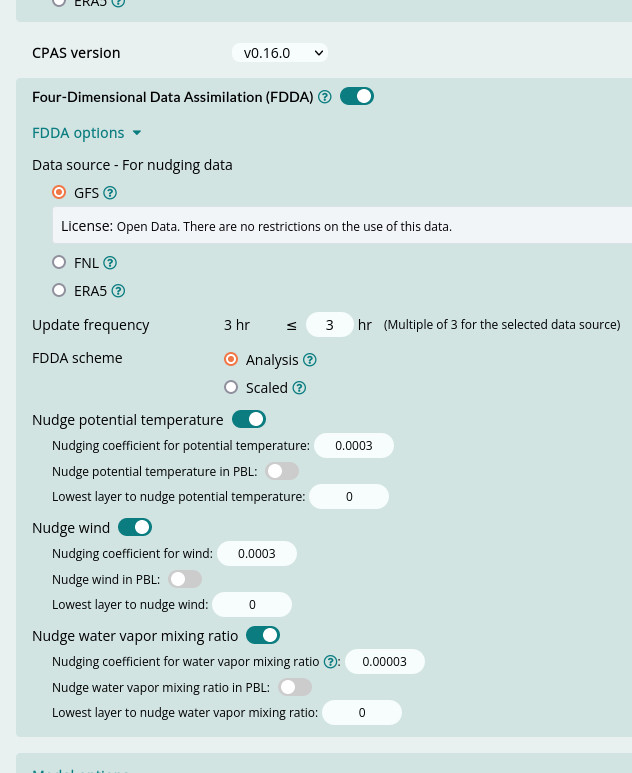
Four-Dimensional Data Assimilation (FDDA) and its options
You can also toggle for the FDDA option. It preserves the variability in the large scale information from the gridded nudging data source. For details, please refer to FDDA option.
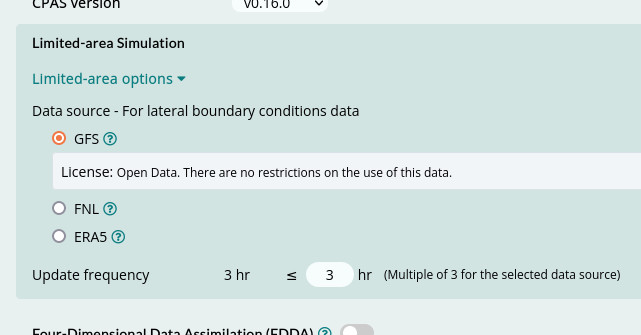
Limited-area simulation
If you define a limited-area domain in the previous mesh specification, there are then options of limited-area simulation for data source of the lateral boundary conditions and its update frequency.
CPAS model options
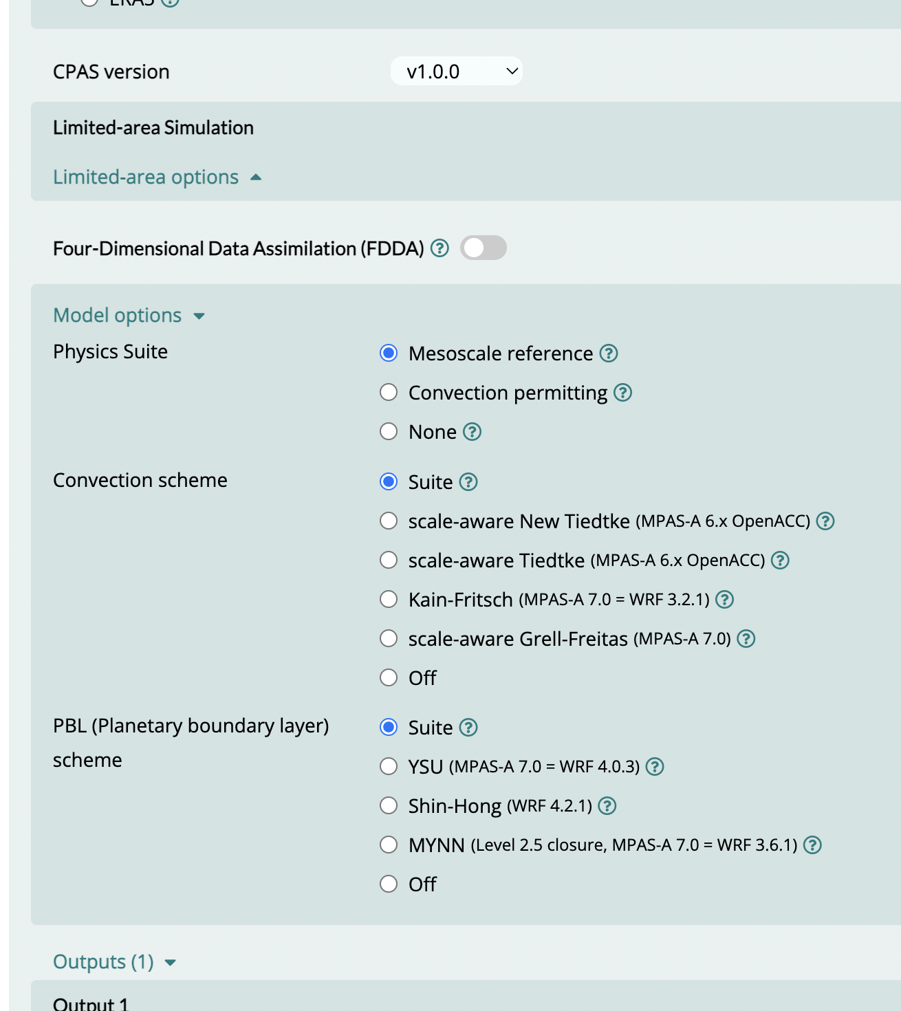
Physics Suites
Please refer to
|
Mesoscale reference |
|
| Convection permitting |
|
| None | All physics parameterizations turned 'off'; intended for idealized simulations. |
Convection schemes
| Suite | Follow the default of the suite. |
| Scale-aware new Tiedtke |
Similar to the Tiedtke scheme used in REGCM4 and ECMWF cy40r1. See:
|
|
Scale-aware Tiedtke |
Mass-flux type scheme with CAPE-removal time scale, shallow component and momentum transport. See:
|
|
Kain-Fritsch |
Deep and shallow convection sub-grid scheme using a mass flux approach with downdrafts and CAPE removal time scale. See:
|
|
Scale-aware Grell-Freitas |
Modified version of scale-aware Grell-Freitas, which is an improved GD (Grell-Devenyi) scheme that tries to smooth the transition to cloud-resolving scales. See:
|
PBL (Planetary boundary layer) schemes
| Suite | Follow the default of the suite. |
| YSU |
Non-local-K scheme with explicit entrainment layer and parabolic K profile in unstable mixed layer. See:
|
|
MYNN |
Predicts sub-grid TKE (Turbulence Kinetic Energy) terms. See:
|
| Shin-Hong |
Include scale dependency for vertical transport in convective PBL. Vertical mixing in the stable PBL and free atmosphere follows YSU. This scheme also has diagnosed TKE and mixing length output. See:
|
Outputs
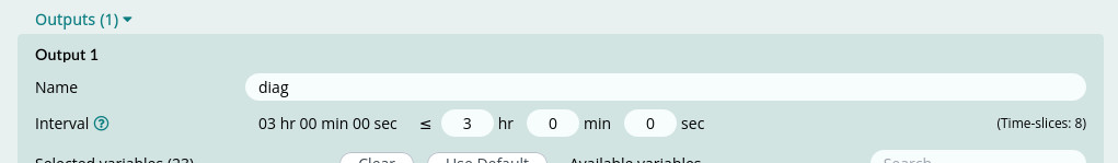
You need to enter a time interval for outputting time-slices of the simulation. It must be a multiple of the time-stepping alignment interval in the mesh generation job. The default time-stepping alignment interval is 30 min which equals the default time interval for running shortwave and longwave radiation parameterization schemes.
|
To change Time-stepping alignment interval of the mesh, you can submit an additional mesh generation job by switching to the “Order Mesh Generation” tab, with:
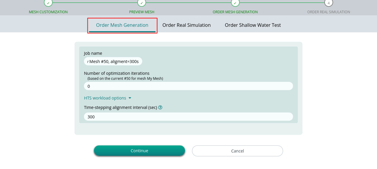 A shorter alignment interval (e.g. 300s), can be used, so that the time interval for outputting time-slices can be shorter accordingly. You may also rename the mesh generation job for your change. |
The total number of time-slices for the output will be indicated at the right of the interval input. For example, 24 hours in length of simulation will produce 8 time-slices, where each adjacent pair of time-slices are separated by a 3-hour interval. For 132 hours in length of simulation, the simulation will produce 44 time-slices of the same 3-hour time interval. It has a proportional impact on the I/O cost.
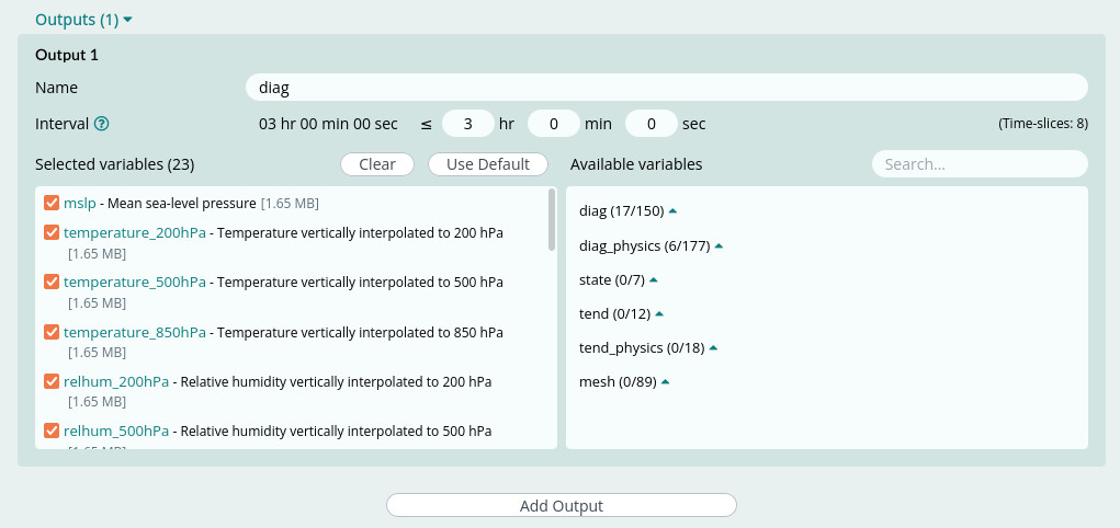
You can choose which variables to output from the running simulation model. There are plenty of choices.
A number of default variables have been preselected on the left panel list. You can deselect or “Clear” all options there, or click “Use Default” to reset the default variables. You can select more available variables from the right panel list, by browsing or searching.
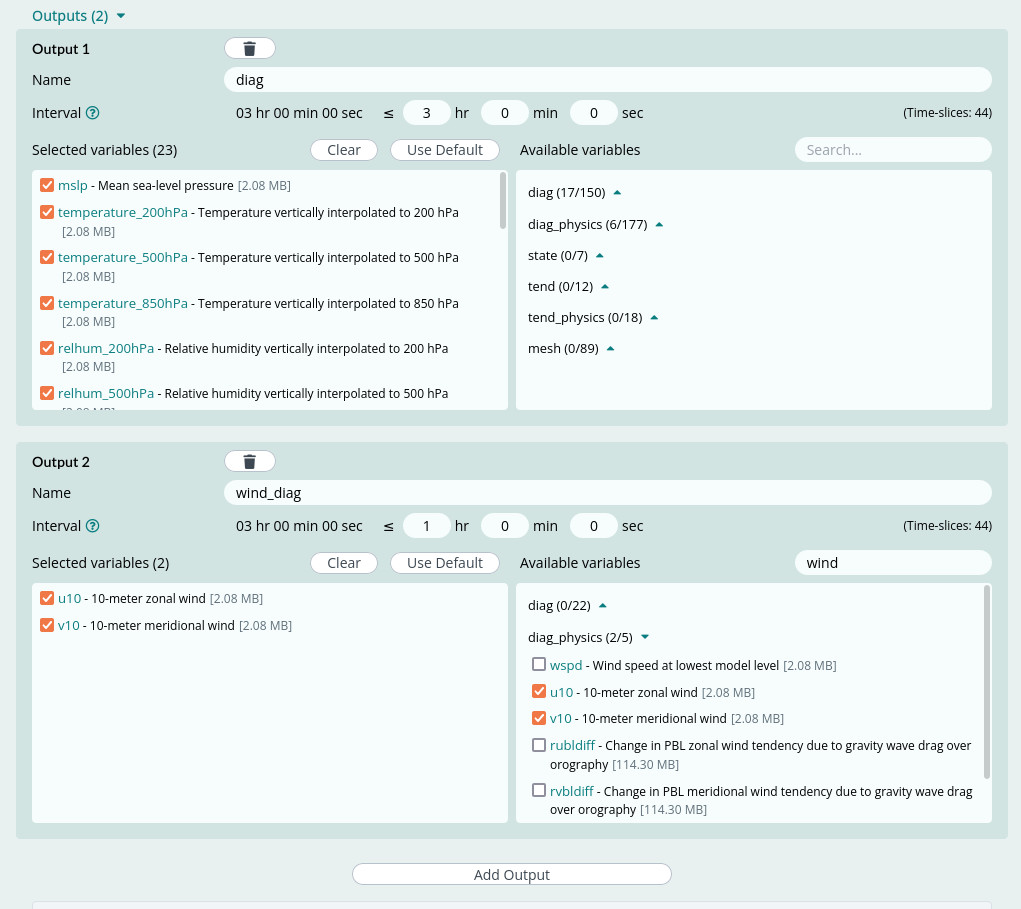
You can also choose to add a second output or more, with a different set of output variables and time interval. Say you want to output common variables in a coarse time interval of 3 hours, while output some wind-related variables more frequently in a time interval of 1 hour. This can save resources in storage and I/O time.
Decide to submit the real simulation job
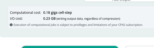
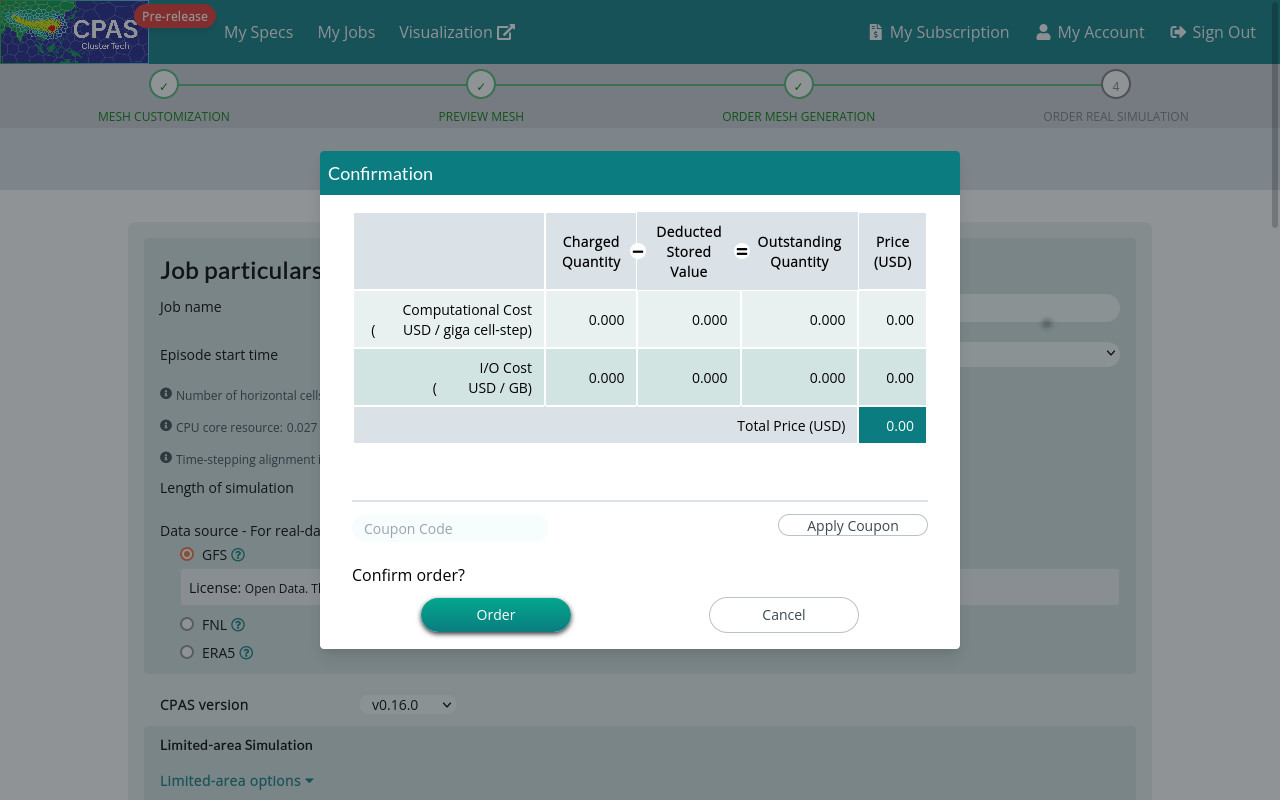
Finally, computation cost and I/O cost are estimated (instantly updated when the settings above are altered). The unit of the computation cost is in giga cell-step (i.e., 109 cell-step), where 1 cell-step represents the average computational cost to compute 1 time step (which is temporal) for 1 mesh cell (which is spatial) during the computational simulation.
If your configuration for the new real simulation is confirmed, you can proceed with the green “Continue” button. Our platform will have a price quotation for you in a modal. If you agree with it, click the green “Order” button to confirm the order. If you have a coupon code, you can enter and apply the code here.
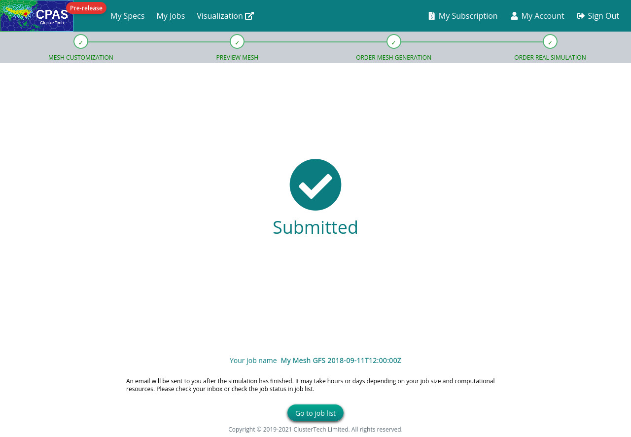
Upon online payment for non-zero price, the new real simulation job is then ordered in our system. It will be queued and run.
Check the status of your new real simulation job
You can check in the “My Jobs” page the current status of your new job, as well as jobs you previously ordered and kept. Click the “Real Simulation” section to see order time, status, storage, etc for all real simulation jobs.
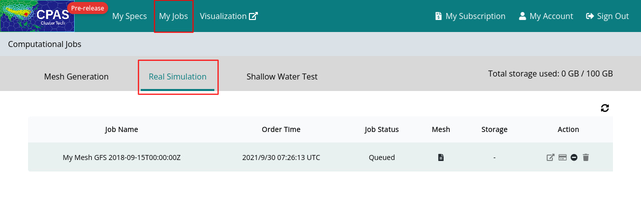
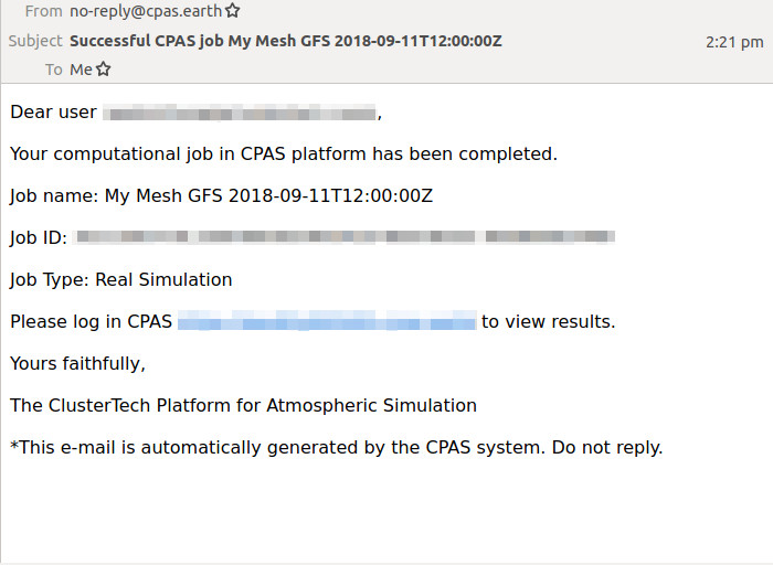
The real simulation job may take a long time to complete, depending on the computational cost. When the job is completed, the 'Job Status' will change from 'Running' to 'Completed', you will then receive a notification email with title prefix 'Successful CPAS job' and suffix of the job name, e.g. 'Successful CPAS job MyMesh GFS 2019-12-22T06:00:00Z'. (If you do not receive the email, check you email Spam folder)
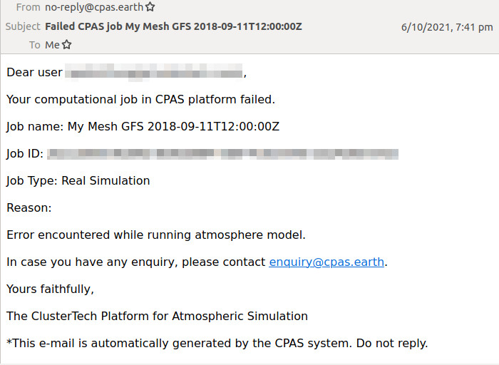
If the job failed, you will receive an email with the title prefix 'Failed CPAS job', in which the Job Status becomes 'Failed'. You can modify the setting based on the hints given in 'Reason' stated in the email if any, and order the real simulation job accordingly. (The Job Name and Order Time help you to identify the failed job)
| Prev | Back to Table of Content |